

 Lavkush
Big O notation tells you how the running time of your code grows as the input grows — and you can learn to read it straight from your own code, step by step. Forget the maths-class fear: Big O is just a label for a growth pattern. One loop over n items is O(n). A loop inside a loop is usually O(n²). Halving the problem again and again is O(log n). This guide teaches you a simple counting method, walks through real Python and JavaScript examples line by line, shows the famous growth chart, and lists the mistakes beginners make most — so next time someone asks "what's the Big O?", you can answer by looking at the code, not by guessing.
We already have a friendly introduction to what Big O notation is on Coding Cush. This post is the practical sequel: less "what is it", more "how do I work it out from this function in front of me".
The One Idea Behind Big O
Big O ignores exact seconds and small details, and asks one question: if the input becomes 10 times bigger, roughly how much more work does the code do? If the answer is "about 10 times more work", that is O(n) — linear growth. If the answer is "about 100 times more", that is O(n²). Exact timings depend on your laptop, your language and the weather in the server room; growth patterns do not. That is why interviews and textbooks care about Big O: it compares ideas, not machines. Khan Academy teaches the formal side of this in its free asymptotic notation lessons, and the Big O notation article on Wikipedia covers the mathematical definition when you are ready for it.
The Step-by-Step Method: Count the Loops
Here is the beginner-friendly method. Step 1: find the loops and recursive calls — they decide almost everything. Step 2: ask how many times each loop runs as n grows. Step 3: loops side by side ADD — keep only the biggest term. Step 4: loops nested inside each other MULTIPLY. Step 5: drop constants and smaller terms, because growth beats details. Let us practise on real code.
def print_items(items):        # one loop over n items
    for item in items:         # runs n times
        print(item)            # constant work each time
# Total: n × constant = O(n)
One loop, n passes, simple constant work inside: O(n). Double the list, double the work. Now the classic trap:
def print_pairs(items):            # find all pairs
    for a in items:                # n times
        for b in items:            # n times, for EACH a
            print(a, b)            # constant work
# Total: n × n = O(n²)
The inner loop does not run n times in total — it runs n times per outer step, so n × n = n² steps. Ten items make 100 pairs; a hundred items make 10,000. That explosion is why O(n²) code feels fine in testing and melts in production.
Halving Means O(log n)
Whenever code throws away half the remaining work each step, the count grows like a logarithm — painfully slowly, in the best way. Searching a sorted list by checking the middle, then the middle of the remaining half, touches about log₂(n) items: 1,000 items need about 10 checks, a million items need only about 20. In JavaScript:
function countHalvings(n) {
  let steps = 0;
  while (n > 1) {
    n = Math.floor(n / 2);   // half the problem each round
    steps++;
  }
  return steps;              // steps grows like log n
}
The pattern to spot is "the problem shrinks by a fraction each round". Half, a third, ten percent — the base of the logarithm changes, and Big O politely ignores that too: it is all just O(log n).
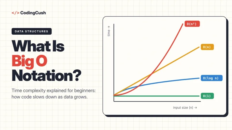
The Chart: Common Complexities Compared
| Big O | Name | Work at n = 100 | Typical example |
|---|---|---|---|
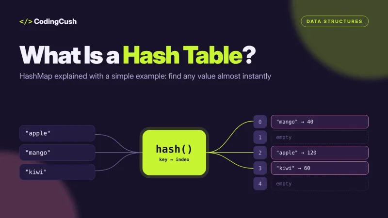
| O(1) | Constant | 1 step | Reading one array index, a hash map lookup |
| O(log n) | Logarithmic | ~7 steps | Binary search in a sorted array |
| O(n) | Linear | 100 steps | One loop, finding a maximum |
| O(n log n) | Linearithmic | ~700 steps | Good sorting: merge sort, quick sort (average) |
| O(n²) | Quadratic | 10,000 steps | Nested loops, comparing every pair |
| O(2ⁿ) | Exponential | More than atoms you can count | Brute-forcing every combination |
Memorise the shape, not the table: flat, gentle curve, straight line, slightly steeper line, wall, rocket to the moon. When you can sketch those six curves from memory, you understand Big O better than many people who use the words daily. Choosing the right structure matters as much as the algorithm — our comparison of array vs linked list shows how the same operation changes cost depending on where your data lives.
Three Worked Examples, Start to Finish
Example 1 — two separate loops. Loop once to find the maximum (O(n)), then loop again to print everything (O(n)). Side by side means add: n + n = 2n, drop the constant: O(n). Two loops do not automatically mean O(n²) — nesting is what multiplies. Example 2 — a loop with a break. Searching a list and stopping when you find the item is still O(n), because Big O describes the worst case: the item might be last, or missing entirely. Example 3 — sorting, then searching. Sort O(n log n), then binary search O(log n). Keep the biggest term: O(n log n). The sort dominates, so optimising the search would be polishing the wrong part.
Mistakes Beginners Make Most
Mistake one: counting lines of code instead of growth — a short function can be O(n²) and a long one O(n). Mistake two: keeping constants, like writing O(2n) or O(n + 5); Big O drops them, so O(n) is the answer. Mistake three: assuming two loops always means n², when only nested loops multiply. Mistake four: using the average case when the question asks for the worst case. Mistake five: forgetting hidden costs — sorting inside a loop, or searching inside a loop, makes that loop much more expensive than it looks. Spot these five and you are ahead of most beginners.
A Quick Self-Test Before You Move On
Try these three in your head. A function that checks only the first element of a list, whatever its size: O(1). A function with one loop that counts matching items: O(n). A function where each item is compared with every item after it — roughly half of all pairs: still O(n²), because half of n² grows like n² once constants are dropped. If you got all three, the method has clicked. If the third one surprised you, reread the drop-the-constants rule — it is the step everyone trips on exactly once.
Frequently Asked Questions
What is the fastest possible Big O?
O(1), constant time — the work stays the same however big the input gets, like reading a known array index. You cannot do better than constant for a single operation.
Why do we drop constants like the 2 in O(2n)?
Because Big O compares growth shapes, not exact counts. As n grows huge, n and 2n have the same shape — a straight line — while n² leaves both behind. Constants belong to timing tests, not growth labels.
Is O(n log n) good or bad?
It is very good — it is the best possible growth for comparison-based sorting, and it scales to millions of items comfortably. Most fast real-world algorithms live at O(n) or O(n log n).
What is the difference between worst case and average case?
Worst case is the unluckiest possible input; average case is the typical one. Big O usually means worst case unless stated otherwise. Quick sort is the classic example: O(n log n) on average, O(n²) in its worst case.
Does Big O measure memory too?
Yes — the same notation describes space complexity: how extra memory grows with input. Copying a list is O(n) space; a few variables is O(1) space.
Conclusion
Reading Big O from code is a skill, not a talent: find the loops, multiply the nested ones, add the separate ones, watch for halving, then drop the small stuff. Practise on your own functions this week and the chart will start reading itself. Slow growth wins — in algorithms and, honestly, in learning them too.

Leave a Comment